Clojure - Linear Regression

We will try to do a basic linear regression here with incanter. If you don't know what linear regression is it is essentially finding the line of best fit. I'll demonstrate how you can find the line of best fit using incanter with a neat function called linear-model which will do a lot of the numerical calculations for us. Make sure to note that the data for the y axis is the first argument and not the second argument since at least for me it appears to be more intuitive to place the x axis in the second argument of the function but that isn't the case for the linear-model function from incanter.stat so take note of that. Let us go ahead and add our dependencies. As well as make sure that incanter is in your project.clj and your namespace looks like the following below.

(ns incantertut.core
  (:use [incanter.charts :only [histogram scatter-plot pie-chart add-points add-lines]]
        [incanter.core :only [view]]
        [incanter.stats :only [sample-normal linear-model]]))
 

What linear-model will do for us will do a bunch of calculations off hand so that we don't have to do them ourselves which is good. However if you are interested in the math computational part like I am you should probably go learn linear algebra and some statistics which will help you understand more of whats going on but it isn't absolutely necessary if you just want a line of best fit to be displayed.

I am not entirely sure why computer science and the machine learning community tend to like to call the line of best fit "linear regression" which sounds a bit scary to me but really all you are doing is fitting a line that happens to be stright to a bunch of points on a x and y axis graph. Nothing complicated really. However when introducing this topic of linear regression in textbooks the impression is that this is a huge big thing but anyways I digress too much and here you go with the easy and simple line of best fit.

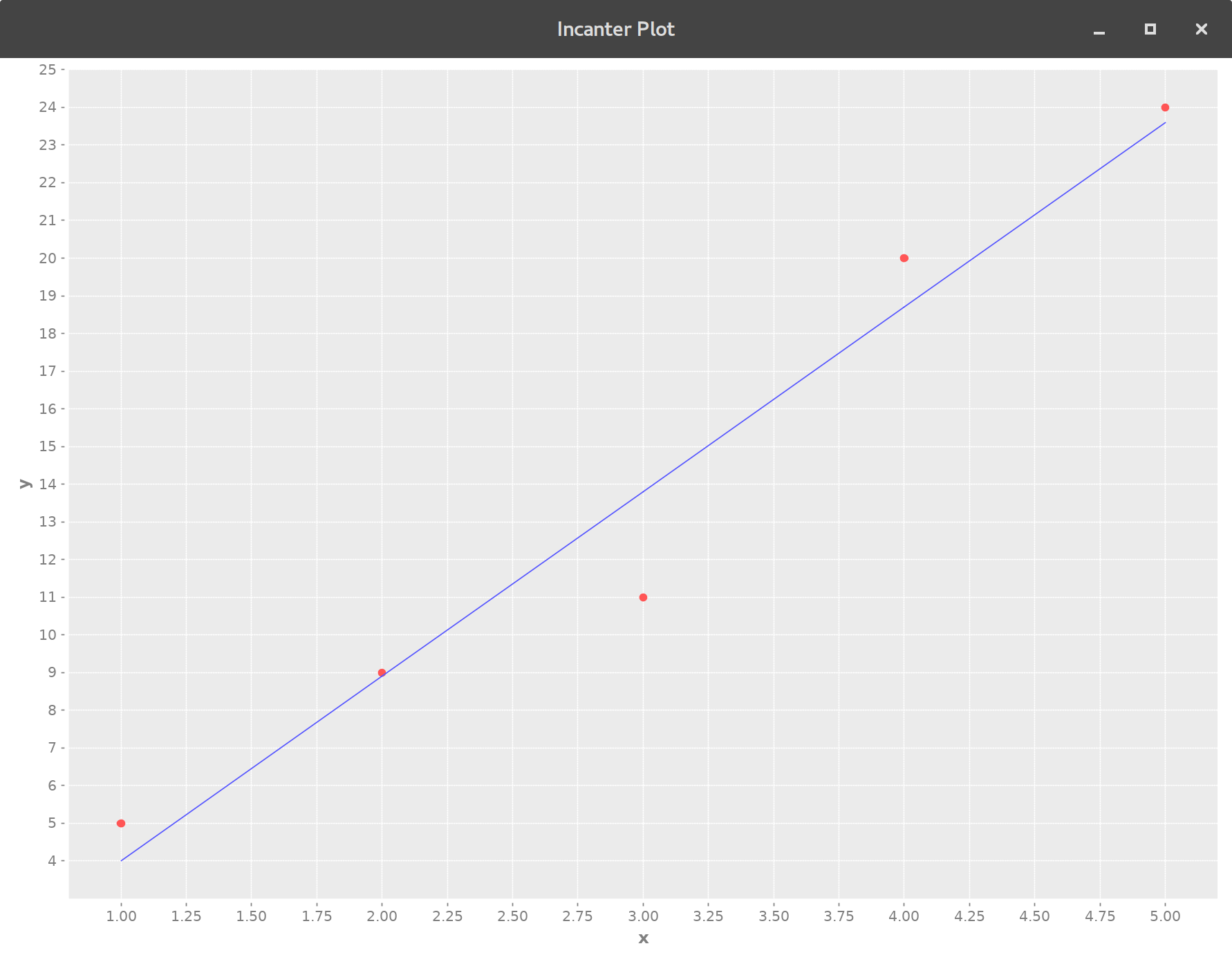
(def x [1 2 3 4 5])
(def y [5 9 11 20 24])

(view (add-lines (scatter-plot x y)
                  x (:fitted (linear-model y x))))
 

Let me go through with what is going on here. The view is again if you haven't read through the previous post on basic incanter on how to display a histogram, scatterplot and a pie chart I suggest looking at that. However I'll assume you know what view is doing and is the function that allows you to see the graphs hence view. The add-lines is a new function from the incanter.charts that I haven't shown before and allows you to plot lines you could use add-points instead as well but than it wouldn't be line.

(:coefs (linear-model y x))
;; => [-0.8999999999999915 4.900000000000002]

Now lets take a look using :coefs gives us two numbers in a persistent vector. So what do those numbers represent? Well one of is negative and the other positive and so judging from the graph you seen the negative number can't be the slope since the slope was clearly had a positive slope. So from that conclusion you can assume that the first number is the y-intercept which it is. The second number is the slope no surprise there.

This is going to be a pretty short post just showing you how to obtain slope and y-intercept but you may not satisfied and be left with questions such as how well fitted is my line of best fit? What is the R² value? How do I get that kind of information from my line of best fit well if you're curious you can check the documentation or wait for the next post.

Tags: Clojure Code Guide

Clojure - R Squared Clojure - Basic Incanter