Clojure - R Squared

We'll pick back up from where we left off in the linear regression post last time. So we'll be keeping pretty much the same dependency of incanter and the name space should still look like the following below more or less.

(ns incantertut.core
  (:use [incanter.charts :only [histogram scatter-plot pie-chart add-points add-lines]]
        [incanter.core :only [view]]
        [incanter.stats :only [sample-normal linear-model]]))
 

We are going to pick up where we left off and find some more interesting properties of the line of best fit such as the r squared value and other properties such as the residuals. So we know that the line of best fit we have which we constructed from the following data ...

(def x [1 2 3 4 5])
(def y [5 9 11 20 24])

(linear-model y x)

(:fitted (linear-model y x))
;; => [4.000000000000011 8.900000000000013 13.800000000000015 18.700000000000017 23.60000000000002]
 

So before getting to the R squared value which we'll get soon enough. Let's look at how far the points are from the line of best fit. To do this incanter has provided :residuals. The residuals are the distance away from the line of best fit. This is useful information to have when trying to understand how well our line of best fit 'fits' the data.

(:residuals (linear-model y x))
;; => [0.9999999999999893 0.09999999999998721 -2.800000000000015 1.299999999999983 0.3999999999999808]
 

So the residuals are nice but maybe you just want to see the absolute distance and not worry about the negatives in the residuals. Easy fix using map to just multiply it with a -1 to make it opposite like so...

(map (fn [x] (if (neg? x) (* x -1) x)) (:residuals (linear-model y x)))
;; => (0.9999999999999893 0.09999999999998721 2.800000000000015 1.299999999999983 0.3999999999999808)
 

Now we have all of the distances as positive lets place them on the graph!

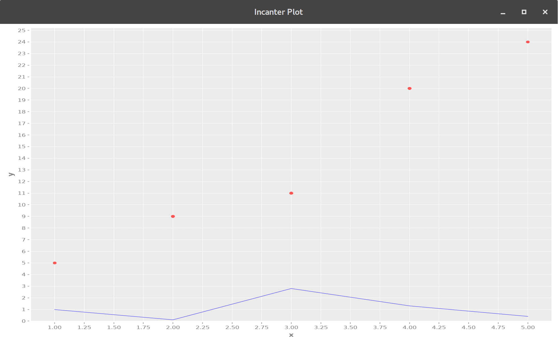
(view (add-lines (scatter-plot x y)
                 x (map (fn [x] (if (neg? x) (* x -1) x)) (:residuals (linear-model y x)))))
 

You'll see somewhat of a representation of those residuals below and seeing from a visual standpoint which datapoints appear to be most out of fit with the line of best fit. Here you can see that the third point seems to be the most nearly 3 units away from the line of best fit.

Now lets do something else with the residuals a common thing to do is that you can square the residuals which will get you the sse or the sum of squares due to error.

(reduce + (map (fn [x] (* x x)) (:residuals (linear-model y x))))
;; => 10.7
 

or actually in incanter you can just do the following instead of typing that entire thing out.

(:sse (linear-model y x))
;; => 10.7
 

So that value gives you some what of an idea of how well the data fits the line of best fit. However we can go and look further and get the R² value from the linear-model.

(:r-square (linear-model y x))
;; => 0.9573365231259969
 

So that is our line of best fit but how well does it fit our data well that is where the R squared value comes in and determines how well our line fits our data. Typically the closer the R squared value is to 1 the better. As well as the R squared value is only ranges from 0 to 1. So 0.95 is pretty good so that our data fits the line of best fit rather well.

Tags: Clojure Code Guide

Clojure - Reading CSV files Clojure - Linear Regression